You run a query that looks perfectly reasonable, but as the table grows larger the response time starts increasing. Someone suggests adding an index. You create one, run the same query again, and suddenly it becomes fast.
At that point most of us accept the result and move on. The common explanation is simply that PostgreSQL uses B-Tree indexes.
But that short explanation hides a lot of interesting details. The structure PostgreSQL uses is not the simple B-Tree you might see in an algorithms textbook. It is a carefully optimized variant designed for disk storage, large datasets, and highly concurrent workloads.
Understanding how it works internally makes many database behaviors easier to reason about. Things like lookup speed, index size, page splits during inserts, and even the performance difference between sequential IDs and random UUIDs all tie back to the way this tree structure is built and maintained.
B-Trees vs B+Trees
Before discussing PostgreSQL specifically, it helps to clarify the difference between a standard B-Tree and a B+Tree.
A B-Tree is a self-balancing search tree where both internal nodes and leaf nodes can store actual data along with keys. When searching for a value, the database might find the result before reaching a leaf node.
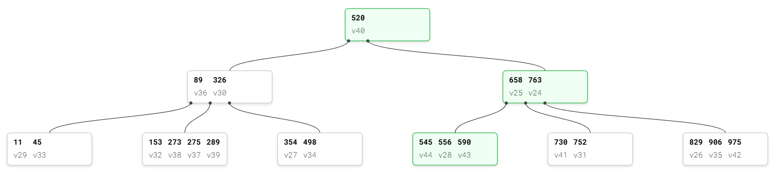
While that sounds efficient, it introduces a problem. Data stored in internal nodes consumes space. Because of this, each node can hold fewer child pointers. That reduces the fanout of the tree and increases its depth.
A B+Tree solves this by separating navigation from storage.
Internal nodes only store keys and pointers, which guide the search path. Actual values are stored only in the leaf nodes.
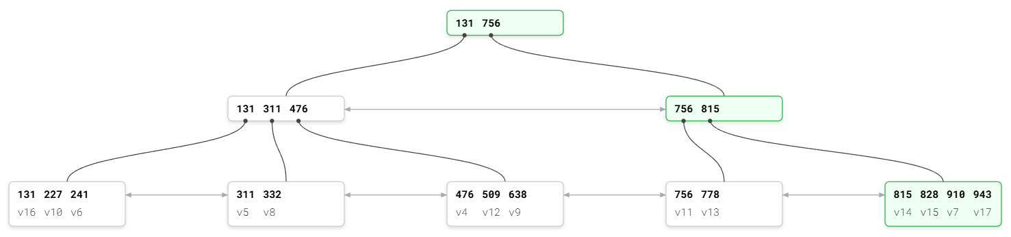
This design increases fanout dramatically. Since internal nodes contain only keys and pointers, they can reference many more children. The result is a much shallower tree, which means fewer disk reads during lookups.
Another important characteristic is that leaf nodes are connected together in a linked list. Once a search reaches the first matching leaf node, the database can simply traverse the next leaf nodes sequentially. This makes range queries extremely efficient.
PostgreSQL’s index implementation is essentially a B+Tree variant.
More specifically, it follows the Lehman and Yao B-Tree algorithm, which allows high concurrency while maintaining correctness during node splits.
If you want to visually understand how these trees behave during insertions and splits, two interactive demos are extremely useful:
You can insert keys and actually see how nodes split and how the tree structure evolves. It makes many of these concepts much easier to understand.
PostgreSQL Index Architecture
PostgreSQL uses a non-clustered storage model.
Tables are stored as unordered heap files, and indexes exist as separate structures that point to rows inside the heap.
Instead of storing the full row, an index entry contains two things:
- the indexed key
- a TID (Tuple Identifier) pointing to the row’s physical location in the heap
This means every index lookup eventually needs to access the heap unless the query can be satisfied entirely from the index.
Both heap pages and index pages use PostgreSQL’s standard 8 KB page size.
Each index page has a structured layout. It starts with a page header, followed by an array of item pointers, free space in the middle, and the stored entries themselves.
Pages are categorized into different node types.
The meta page is stored at block 0 and contains metadata about the index, including a pointer to the root node.
The root node acts as the entry point for every search operation.
If the index grows larger, intermediate internal nodes appear between the root and the leaves. These nodes contain separator keys that define ranges handled by their child nodes.
Finally, the leaf nodes store the actual indexed keys along with TIDs pointing to heap rows.
Because internal nodes only store keys and pointers, they can reference a very large number of children. This gives B-Trees extremely high fanout.
With PostgreSQL’s page size, a leaf page might store roughly 300 entries, while an internal page may point to around 600 children.
This leads to surprisingly small tree depths.
A tree with only two levels, meaning root and leaves, can index around 180,000 rows.
Add one more internal level and the tree can cover more than 100 million rows.
Even at massive scale, most lookups require only a few page reads.
How Searches Work
Every index lookup begins at the root node.
Inside each node, PostgreSQL performs a binary search among the stored keys to determine which child pointer to follow. This process repeats until the search reaches a leaf node.
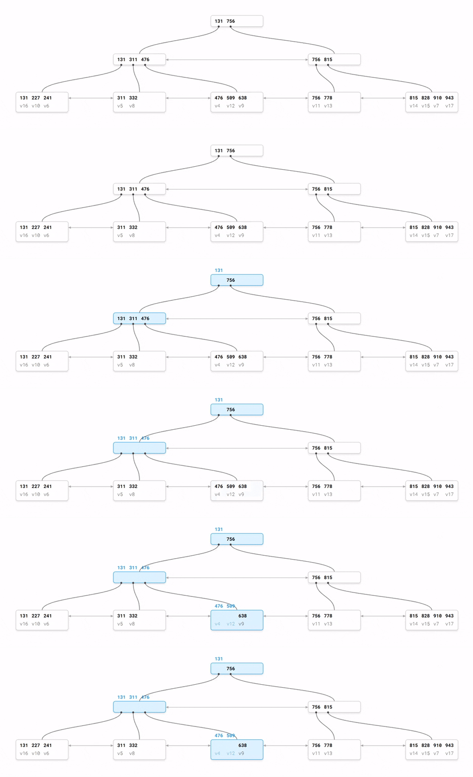
Once the correct leaf page is located, another binary search finds the exact key. The associated TID tells PostgreSQL where to locate the row in the heap.
If the query is a range query such as WHERE price BETWEEN 100 AND 200, the database finds the starting key and then simply walks the linked list of leaf pages to collect matching entries.
This linked structure is one of the main reasons B+Trees work so well for ordered queries.
Insertions and Node Splits
Indexes constantly change as new rows are inserted.
When a leaf node has enough space, the new key is simply inserted in sorted order.
But when the page becomes full, PostgreSQL performs a node split.

A new page is allocated. Roughly half the entries from the original page are moved to the new page. The split boundary key is then inserted into the parent node to maintain the correct tree structure.
If the parent node also becomes full, the split propagates upward.
In the rare case where the root splits, PostgreSQL creates a new root and increases the height of the tree.
This process ensures the tree always remains balanced.
Deletions and Node Merges
When rows are deleted, leaf pages can become underutilized.
If the number of entries in a node falls below a certain threshold, PostgreSQL may merge the node with its neighboring sibling.
This removes the separator key from the parent node and consolidates the entries into a single page.
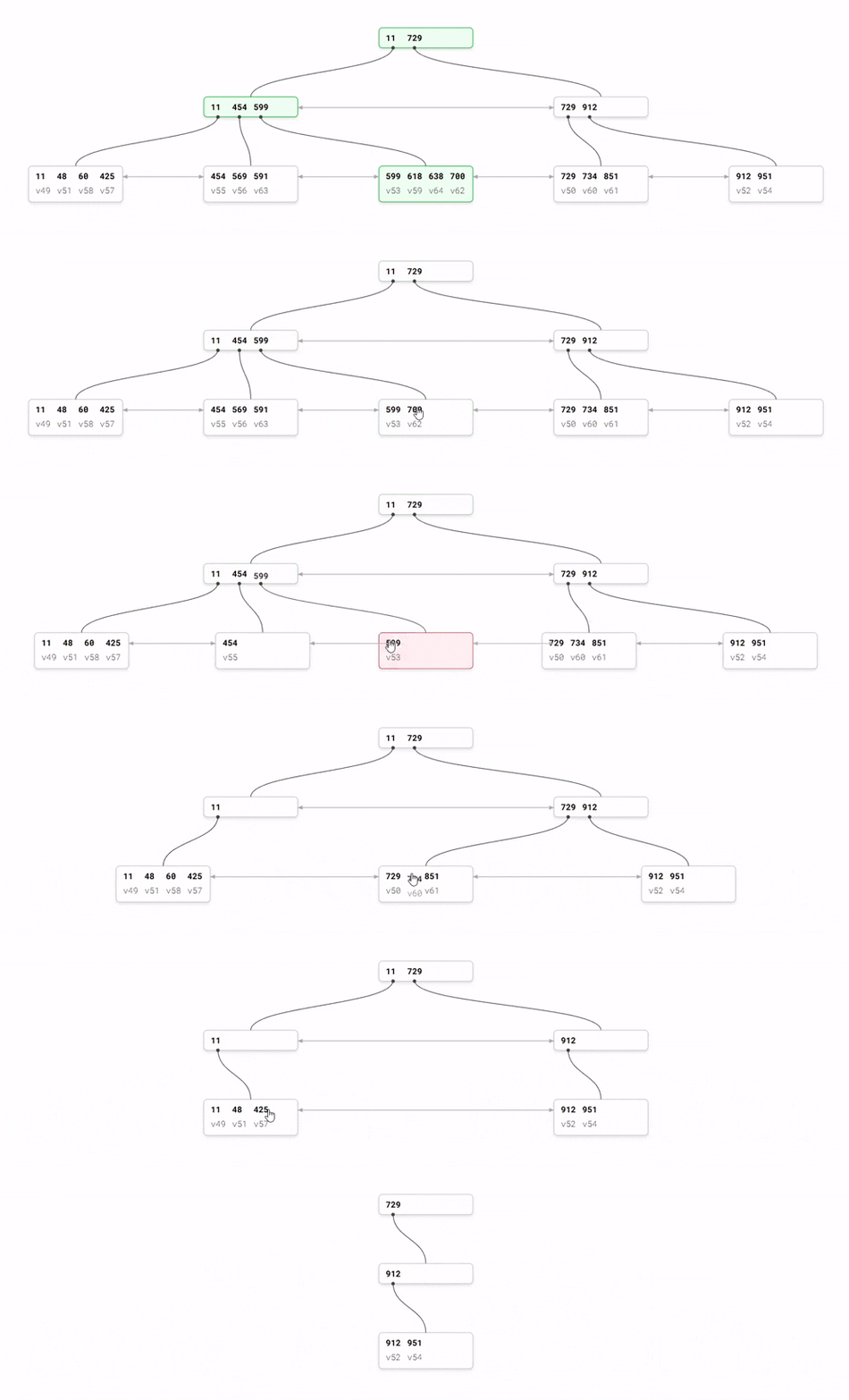
These operations maintain efficient page utilization and prevent the tree from becoming sparse.
Deduplication for Duplicate Keys
One interesting optimization introduced in PostgreSQL 13 is index deduplication.
In earlier versions, if many rows had the same indexed value, the index stored that value repeatedly with different TIDs.
Columns with low cardinality such as status flags could create extremely large indexes.
With deduplication, PostgreSQL stores the key once and attaches a compact list of TIDs that share the same value.
This significantly reduces index size and improves cache efficiency, especially for highly duplicated columns.
Index-Only Scans
Normally, using an index requires two steps.
First the index identifies matching TIDs. Then PostgreSQL fetches the actual rows from the heap.
But sometimes the query only needs columns that already exist in the index.
In that case PostgreSQL can perform an index-only scan.
The only complication comes from MVCC visibility rules. PostgreSQL must ensure that the row is visible to the current transaction.
To avoid heap access, PostgreSQL checks the visibility map, which tracks whether a heap page contains only visible rows.
If the page is marked all-visible, PostgreSQL can return the result directly from the index.
To support more index-only queries, PostgreSQL allows additional columns to be stored using the INCLUDE clause. These columns are stored only in leaf nodes so they do not increase the size of internal nodes.
Multicolumn Indexes and Skip Scans
Multicolumn indexes follow a strict ordering.
For an index like (a, b), queries filtering on a benefit the most because a determines the primary ordering of the index.
Queries filtering only on b usually cannot use the index efficiently.
However, PostgreSQL can sometimes perform a skip scan.
If column a has very few distinct values, the planner can iterate through each possible value of a and search for matching b values within those partitions.
This technique is not always used, but when applicable it allows the database to use an index that might otherwise seem unusable.
Combining Multiple Indexes with Bitmap Scans
PostgreSQL can also combine multiple indexes for complex conditions.
Suppose a query contains several predicates such as:
WHERE status = 'pending'
AND created_at > NOW() - INTERVAL '1 day'
Instead of choosing only one index, PostgreSQL may perform bitmap index scans.
Each index scan produces a bitmap representing matching heap locations. These bitmaps are then combined using bitwise operations like AND or OR.
Once the final bitmap is constructed, PostgreSQL reads the heap pages in physical order. This reduces random disk I/O and improves performance for large result sets.
Choosing Good Index Keys
Index design choices can significantly affect performance.
One common example is the difference between random UUID keys and sequential integers.
Random UUIDs distribute inserts across the entire B-Tree. This leads to frequent page splits, fragmentation, and poor cache locality.
Sequential keys behave very differently. Inserts always occur at the rightmost leaf page. Pages fill sequentially and remain densely packed.
This pattern minimizes page splits and improves buffer cache efficiency.
Another useful technique is the partial index.
If queries consistently target a small subset of rows, the index can be created with a condition. Only rows satisfying that condition are indexed.
For example, if an application frequently queries unprocessed jobs, an index on only those rows can remain extremely small and efficient.
Why This Matters
B-Tree indexing in PostgreSQL is a good example of how theoretical data structures evolve in real systems.
The core idea remains simple. Maintain a balanced tree so that lookups require only a few comparisons and page reads.
But the actual implementation includes many additional considerations such as concurrency control, page layout, MVCC visibility, and disk I/O patterns.
Understanding these details helps explain many real world behaviors in PostgreSQL. It also helps when deciding how to design indexes, choose key types, and interpret query plans.